Example on the Maroni basin, French Guyana
- Building the coupled model
The hydraulic and hydrological model are first built separately, each according to available data and to the scale of the modeled processes. Here, we will focus mostly on building the hydrological model (see also our “How to use satellite data to build a hydraulic model” news series”).
The hydrological model is a spatially distributed GR4-like model (see SMASH documentation and [1]). grid is built based on a 30s resolution flow direction map. Model forcings are provided by GSMaP precipitation product (debiased using IMERG Late V07 and Quantile Mapping [2]) and ERA5 evapotranspiration data (both on coarser 10×10 km² grid, daily time steps). Correspondence between the hydraulic and hydrological grids is obtained by I) selecting all hydrological pixels downstream form the upstream-most hydraulic points (using the flow direction map), checking their closeness to the SWORD centerline (used to build the hydraulic model), then assigning each hydrological cell to the nearest hydraulic cross-section [3]. Mass source terms are used to inject the distributed hydrological discharge hydrographs into the hydraulic model at all identified coupling points
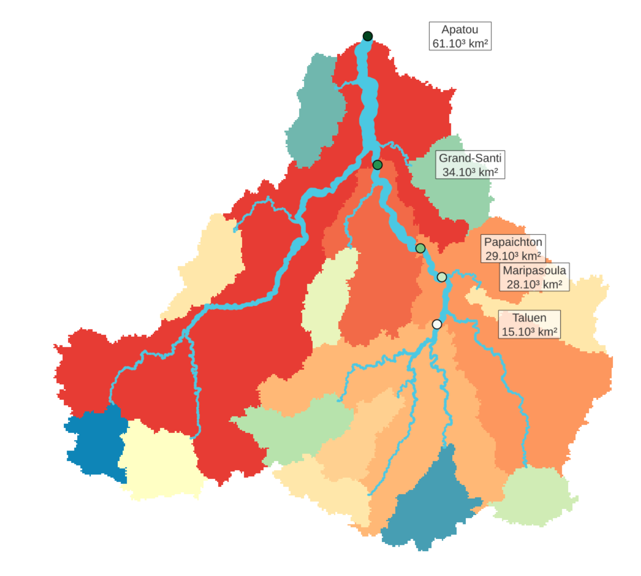
Finally, the parameters of the hydrological model are defined as homogeneous over 16 user-defined regions. Each region is defined as the catchment upstream of either one of the in situ gauges – where already available data carries information – or one of the upstream boundary points of the hydraulic model – where information obtained by calibrating the hydraulic model will be backpropagated toward the hydrological model. This step is necessary to ensure that the inverse/calibration problem is not over-parameterized, while still providing sufficient freedom to the assimilation process to fit observed data.

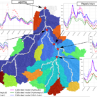
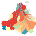
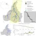
Figure 1: The Maroni basin. Green dots: locations of in situ gauges gathering real data. Cyan: hydraulic model extent and width (8000+ cross sections, 1600+ coupling points). Colored regions: regionalization of the (finely) distributed hydrological parameters into 16 homogeneous zones, based on available information density.
In the next and last part of this series, we will look at some calibration results that this H&H framework can provide, specifically by assimilation SWOT altimetry data. Significant coupled model performance improvements can be achieved thanks to informative assimilated observation and analysis of the inverse/calibration problem that is solved.
[1] Colleoni, F., Huynh, N. N. T., Garambois, P.-A., Jay-Allemand, M., Organde, D., Renard, B., . . . Javelle, P. (2025). Smash v1.0: A differentiable and regionalizable high-resolution hydrological modeling and data assimilation framework. EGUsphere, 2025 , 1–36. doi: 10.5194/egusphere-2025-690
[2] Cannon, A. J., Sobie, S. R., & Murdock, T. Q. (2015). Bias correction of gcm precipitation by quantile mapping: How well do methods preserve changes in quantiles and extremes? Journal of Climate, 28 (17), 6938 – 6959.413. doi:10.1175/JCLI-D-14-00754.1
[3] Berkaoui M.A., Saadi M., Colleoni F., Huynh T., Akhtari A., Larnier K., Garambois P.-A., Roux H. (in redaction). A Raster–Vector Framework for Multi-Scale Hydrological–Hydraulic Modeling Across Large Domains